Go To Special
Have you ever subtotaled data or produced a pivot table and wanted to use the summarized information for further calculations? Normally if you copy filtered or subtotaled data, all the data, including the hidden rows, is copied.There is an easy way around this. It’s in the Go To Special feature of Excel and the option is labeled Visible cells only.
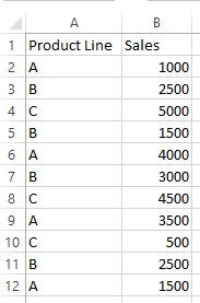
Assume that you have the following simplified data:
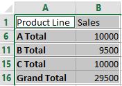
First, use subtotal to accumulate the sum of sales by product line. After sorting the data by product line and using the subtotal feature, the following is obtained:
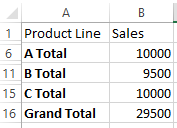 As you can see, the subtotaled data hides some columns. Continuing to work with the subtotaled data may cause a mess, especially if you want to create a new subtotal.
An easy way around this issue is to copy the data. If a basic copy/paste was performed in an area that wasn’t within the same set of rows on the worksheet or was on another worksheet, you would have all the detail data rather than just the summarized data. However, you can avoid this by using the Go To Special feature and the Visible cells only option.
First, select the subtotaled data. 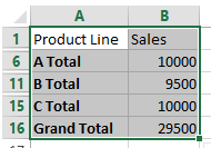
Next, click on Find & Select in the Home ribbon and select Go To Special.
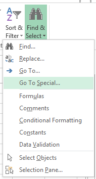
When Go To Special has been selected, a dialog box appears with more options.
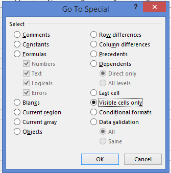
Select Visible cells only, then click OK.
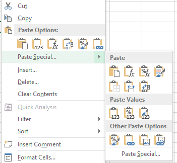
Notice that each cell now appears to be highlighted by a box. Right click anywhere in the area and select copy. The box highlights around each cell appear as if they’re moving. Right click on cell A20 and select Paste Special then Values (This is important. It tells Excel to only paste the values in the cells rather than the formulas.)
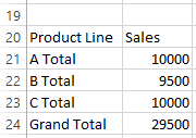
 After the Values option has been selected from Paste Special, the summarized data, without all the detail, is now available to work with.
I use this technique a lot with pivot tables. Many times, I want to reference a summarized column of information on a pivot table for subsequent calculations. This can be done with pivot table data. However, if the pivot table is large and you want to copy formulas involving pivot table data, it’s not always easy as pivot table data contains absolute cell references (eg. Copying a formula down that contains the first piece of summarized information in a pivot table will continue to only use the data in that first cell.)
So, if I want to work with pivot table data, I generally isolate the visible cells using Go To Special, then copy only the visible cells and use Paste special-Values to copy the data to another worksheet and perform further analysis.