I should not even be telling this story but here goes. My husband took an Excel course yesterday and came home all excited to share the tips he learned. Yes, I too wondered why he was taking an Excel course when he could ask me a question or better yet – read my blog or eBooks! Anyway, I digress.
Sadly, the two tips he learned have been around forever. I could not believe that he did not already know them since he has been using Excel since 1995. When I mentioned this, his response was that many people do not know these tips or learn them and then forget about them if they are not using them frequently. After some thought, I realized he might be right. So, here is a list of my favorite tips. I hope that you find at least one new tip that you did not know before.
My Top Tip: Copying Hidden Rows and Subtotals
Mr. Excel actually included my tip in his last book – “The 40 Greatest Excel Tips of All Time”.
I use this feature almost every day. If you have hidden data or have subtotaled data, when you copy it, Excel copies ALL the data in the selected area. If you just want to copy and paste what you can see, select your data, go to Find & Select (or use the F5 key) and then click on Go to Special. Select Visible Cells Only and click OK. Now copy your data and you will see a strobe effect around the data. Paste it and Excel will only paste the visible cells in the data range that you selected. If it doesn’t work, chances are you forgot to copy – something I do all the time.
The good news is that in newer Excel versions, if you copy filtered data, Excel will automatically copy just the filtered data. For subtotals and hidden data, you still need to do this workaround.
My Favorite Navigation Tip
This is my favorite navigation tip. I am one of those people who has way too many files and can never find the one I need immediately. I have a couple of key files that I frequently reference, so I pinned them. When you PIN the file, it will display at the top of the file list. This also works in Word as well. As you pin more files, the first ones move down the most recently used list; however, they will not disappear until you unpin them. The pin turns green to show it is pinned. It turns gray if you click on it and unpin it.

Just open Excel look for a file and you will see the Pin icon over on the right. You can also search for Recent files as well as Pinned files. This can save you hunting through folder after folder for that budget you put together a few months back.
Tips Joe learned:
Double-click a Column to Copy a formula down

In this example below, Cell F7 (Total Sales) is a calculation. It is multiplying the Price/lb. (D7) and Quantity Sold (E7). Once I have the formula in F7, I can double-click the lower right-hand corner of F7 and Excel will automatically copy the formula down to all the other cells until it finds a blank row. This is a big timesaver.
F4 Key
F4 repeats the last action unless it is typing. It is similar to the format painter button. So, if you just formatted the top row of your income statement with the currency symbol. Select the bottom row and press F4. It will apply the symbols for you to the selected area.
Did you know that if you click the Format Painter button twice, it will repeat the last action repeatedly until you click the Format Painter button again? This also works in Word. This is my tip as apparently Joe did not learn that yesterday. Sour grapes? Maybe.
By the way, the F4 key also allows you to cycle between relative and absolute cell references if you are working in a formula. It saves you dealing with typing in or removing dollar signs.
Other Fun Tips
Key Short Cuts
Selecting Data
- If you’ve selected too much or too little, simply hold down the Shift Key and then use the arrows on the keyboard to add or reduce cells. The Shift Key locks you into place. This also works in Microsoft Word.
- Selecting Non-Contiguous Cells
- Select the first cell or range of cells that way you normally would.
- Then hold down the CTRL key and select the next cell or range of cells.
- If you have another row, select it (still holding down the CTRL key)
- Deselect the CTRL key when you have finished.
This is useful for formatting and for auto summing multiple columns of data.
Name Box
for Nested Formulas
The Name Box is extremely useful if you want to nest formulas using different functions. Create your first formula using a function and then when you need the next function instead of typing it in, click the drop-down arrow in the Name Box and select the function.

For Range Names
To create a range name, the fastest way is to type it in the Name Box.
Custom Sorting
If you have sales offices or product lines and you need to sort their data you might be interested in custom lists. Custom Lists allow you to sort data the order you want instead of alphabetically. Let’s say your list of sales offices is Boston, New York, Chicago, Atlanta, Dallas, Los Angeles and you want to display them in that order rather than have them sort alphabetically.
Click the Sort button.
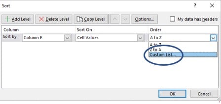
Select Custom list from the Order drop-down.
Click New List and then in the second column, type the entries in one per line in the order you want them to sort.
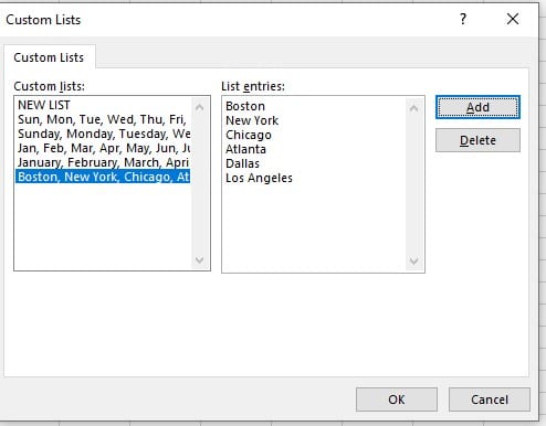
Click Add.
Click OK.
Now select your data and select Custom List in the Sort dialog box. Select the list you want and click OK.
Excel will sort the data in your Custom List Order. You only have to do this once and Excel will remember this for all your files. One caveat, Excel will default to that custom list and try to sort on it next time you sort data even if it does not contain anything on the list.
Don’t have access to two monitors?
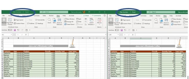
A lot of people today have two monitors which makes things much easier but if you have a boss who won’t spring for a second monitor, you can create a duplicate of the file you are working on so you can view more than one worksheet in the file at a time. So, if you want to view 2 or more worksheets at the same time on your computer screen all you have to do is open a second window.

Select the View Tab and then in the Window group, click New Window.
It doesn’t look like anything happens when you do this however if you look up at the title bar, you will now see a :2 after the file name to show that a second copy (window) has been made.
Select Arrange All to display them the way you want. You can then use each window to display and edit different parts of the same workbook.
The files are mirror images of each other and any change is actually appearing in both at the same time. This can be very useful if you want to copy something or are creating formulas.
This trick was a favorite of mine until I purchased a second monitor and hooked them together so that I can now easily move between different sheets or files.
Tip: Close out the :2 version first and then you will see the :1 disappear from the original. If you close out the :1 first, it is not a big deal, however you will always have that :2 after the name and then you are always wondering whatever happened to Version 1.
Copying the Same Information onto Multiple Sheets at the Same Time
If you do budgets or any type of analysis of multiple departments or sales areas, this tip will blow your mind. The “technical” name for this feature is Grouping. For example, let’s say you are responsible for 5 sales regions and need to create 5 budgets. With grouping, you can create all 5 budgets at the same time.
- Make sure that you have 5 sheets in the file.
- Right-click on any sheet tab and then click on Select All Sheets.
- The word Group now appears beside the file name at the top of the file.
- Everything that you do, including formatting, will now automatically replicate on all 5 sheets at the same time. Pretty neat!
- Right-click on the sheet tab to Ungroup the sheets when you are finished.
The reason this is so useful is that if you created a budget and then copied it to the other sheets you would still have to go in manually and adjust column widths and some other formatting. With grouping, you don’t have to worry about that as all the sheets are set up identically.
It is very important to ungroup. Too often people forget and then start overwriting data so make sure to ungroup your sheets!
If you need to go in and fix a formula or add something after the fact, just group them again and edit the information once. Grouping is also useful if you want to print a lot of sheets.
Create Nested Subtotals
I showed this tip to a class at the Indiana CPA Society and a woman came up after class and told me that if she had taken the class a week earlier, she could have saved herself about 8 hours of work.
If you want to create a nested subtotal, begin by creating your first subtotal as you normally would. Then, go back into the Subtotal dialog box to create a second subtotal. For instance, I could go back into the dialog box and select Average if I wanted to see both Total and Average units sold. Before clicking OK, make sure to uncheck the Replace current subtotals option. Removing that checkmark ensures that the original subtotals are not overwritten.
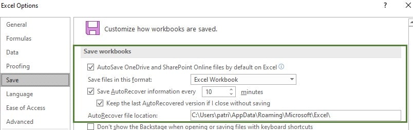
Recover Unsaved Workbooks
I am going to end with this tip as it seems appropriate- How to Recover unsaved Workbooks.
This feature is automatically turned on in Excel 2010 and higher. In later versions, you can also autosave files that you are working on in OneDrive.

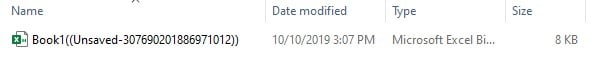
Say, it’s Friday night and almost 5, so you click that Don’t Save button one too many times because you are in a hurry and suddenly you have that sick feeling in the pit of your stomach. Good news. You can still make that evening soccer game because you don’t have to recreate the file. Open Excel and look at the bottom of the screen under the existing file names and you should see:

Click Recover Unsaved Workbooks and it will display the unsaved workbooks.
If you have an earlier version, you may have to select Open Other Workbooks before you see the Recover Unsaved Workbooks.
Once you find the file, Open it and then select Save As.