Gantt Chart using Excel

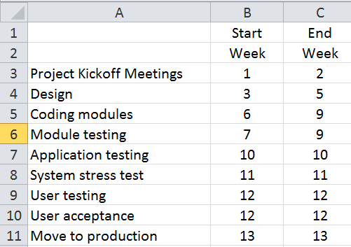
A Gantt Chart is used in project scheduling.  It takes each activity and provides a sideways bar to visually show when that activity occurs within the total project.Excel can be used for Gantt Charts using the IF function, the AND function and Conditional Formatting.  Assume that your project consists of the following:

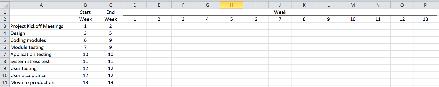
To continue the chart, add the weeks to the right that will be used to represent which project activity occurs during each time period.

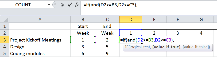
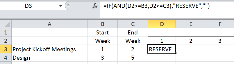
The IF function can be used to determine in which week(s) an activity occurs.  Using the first activity, we want to know if Week 1 in cell D2 is both greater than or equal to the start week in cell B3 and less than or equal to the end week in cell C3.  Put in plain English, we want an IF function that says IF D2 >= B3 AND D2 <= C3, then do something. Fortunately, Excel has an AND function that can be combined with the IF function.  The syntax for the AND function is =AND(logical 1, logical 2, logical 3, etc.)  In this case, the AND function would be =AND(D2>=B3,D2<=C3).  This says that the 1 in cell D2 must be both greater than or equal to the 1 in cell B3 AND less than or equal to the 2 in cell C3. When the above is paired with the IF function, it looks like this:

Now, we need to know what to do if the IF condition is TRUE.  In this example, let’s put the word “RESERVE” in the cell.  It can be any word or number, as long as it is consistent.  If the condition is FALSE, let’s put a blank in the cell.

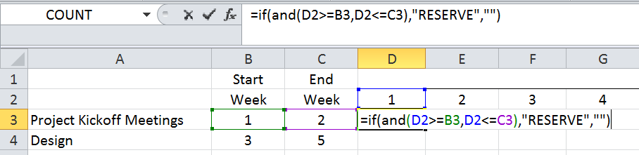
Press enter.

Now, it would be nice to copy this formula.  However, when a formula is copied, the cell references are relative.  This means that if the formula in D3 is copied down to D4, all the row references are adjusted down one row.  If that happens, we’re no longer comparing the 1 in cell D2.  Now, we’re comparing to the IF function in cell D3.
To overcome this problem, Excel allows us to use absolute cell references.  Absolute cell references hold a particular row or column (or both) in place when formulas are copied.  It is done using a $ sign in front of the row and/or column being used in the formula.
In this case, if the formula is copied down, we know that we always want the amount in row 2 and also always want the amounts in columns B and C.  Put a $ sign in front of the 2 in D2 and in front of the references for columns B and C.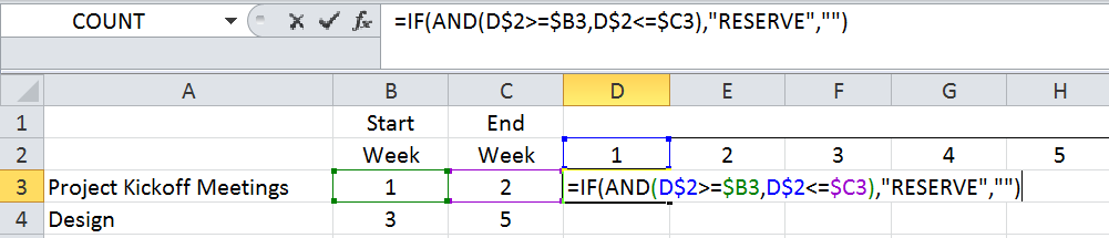

Press enter.  Copy the down to the end of the activities.

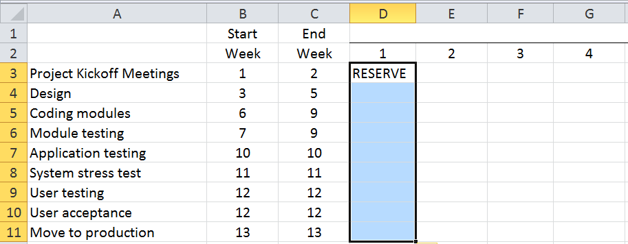
Now, with the range D3:D11 selected, grab the lower right corner with your mouse (you should see a plus sign), click and drag over to column P.

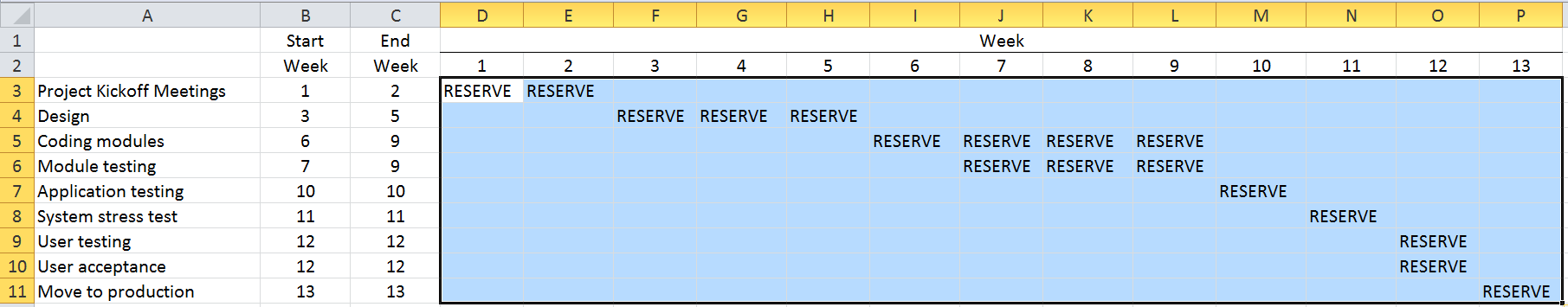
Give it the sanity test to make sure that where the word RESERVE is reflected that it represents a scheduled activity. While this would work, it’s not a real Gantt Chart.  A Gantt Chart uses horizontal bars to reflect a scheduled activity.  This is where the Conditional Formatting is used.Conditional Formatting will color the contents of a cell or the entire cell based on a defined condition.  In this case, we’re going to color the entire cell black if it contains the word RESERVE.Keep the area D3:P11 selected.  Click on Conditional Formatting in the Home ribbon at the top of the screen.  Then, click on Highlight Cells Rules, then click on Equal to.  The following dialog box will appear: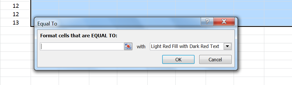

 

In the EQUAL TO: box, type RESERVE.  In the drop down box following “with”, click on the drop down arrow and select custom format…
Select the Fill tab and then select the color black for the color options.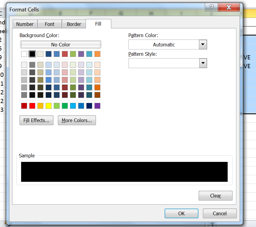 

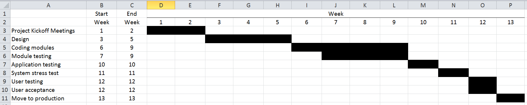
Click OK.  Click any other area of the spreadsheet to deselect the range and your Gantt Chart is ready for use.

 

It’s an easy way to create a Gantt Chart without special software.  You just need to know the IF function, the AND function, and Conditional Formatting.  We also covered absolute cell references to make it easier to copy the formulas down and across.